Interrupted Time Series (ITS) with scikit-learn models#
This notebook shows an example of using interrupted time series, where we do not have untreated control units of a similar nature to the treated unit and we just have a single time series of observations and the predictor variables are simply time and month.
import pandas as pd
from sklearn.linear_model import LinearRegression

import causalpy as cp
%config InlineBackend.figure_format = 'retina'
Load data#
df = (
    cp.load_data("its")
    .assign(date=lambda x: pd.to_datetime(x["date"]))
    .set_index("date")
)

treatment_time = pd.to_datetime("2017-01-01")
df.head()
| month | year | t | y | |
|---|---|---|---|---|
| date | ||||
| 2010-01-31 | 1 | 2010 | 0 | 25.058186 |
| 2010-02-28 | 2 | 2010 | 1 | 27.189812 |
| 2010-03-31 | 3 | 2010 | 2 | 26.487551 |
| 2010-04-30 | 4 | 2010 | 3 | 31.241716 |
| 2010-05-31 | 5 | 2010 | 4 | 40.753973 |
Run the analysis#
result = cp.InterruptedTimeSeries(
    df,
    treatment_time,
    formula="y ~ 1 + t + C(month)",
    model=LinearRegression(),
)
Examine the results#
fig, ax = result.plot()
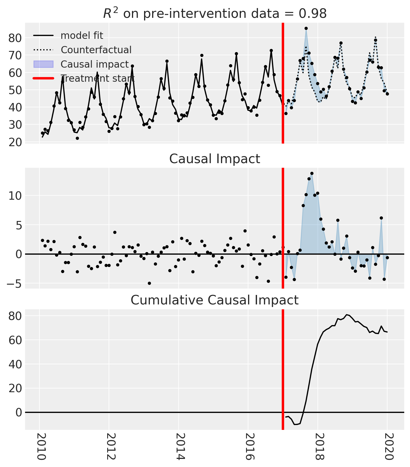
result.summary(round_to=3)
==================================Pre-Post Fit==================================
Formula: y ~ 1 + t + C(month)
Model coefficients:
  Intercept     	         0
  C(month)[T.2] 	      2.85
  C(month)[T.3] 	      1.16
  C(month)[T.4] 	      7.15
  C(month)[T.5] 	        15
  C(month)[T.6] 	      24.8
  C(month)[T.7] 	      18.2
  C(month)[T.8] 	      33.5
  C(month)[T.9] 	      16.2
  C(month)[T.10]	      9.19
  C(month)[T.11]	      6.28
  C(month)[T.12]	     0.578
  t             	      0.21
Effect Summary Reporting#
For decision-making, you often need a concise summary of the causal effect. The effect_summary() method provides a decision-ready report with key statistics.
Note
OLS vs PyMC Models: When using OLS models (scikit-learn), the effect_summary() provides confidence intervals and p-values (frequentist inference), rather than the posterior distributions, HDI intervals, and tail probabilities provided by PyMC models (Bayesian inference). OLS tables include: mean, CI_lower, CI_upper, and p_value, but do not include median, tail probabilities (P(effect>0)), or ROPE probabilities.
# Generate effect summary for the full post-period
stats = result.effect_summary()
stats.table
| mean | ci_lower | ci_upper | p_value | relative_mean | relative_ci_lower | relative_ci_upper | |
|---|---|---|---|---|---|---|---|
| average | 1.845561 | 0.161437 | 3.529686 | 0.032645 | 3.366709 | 0.150601 | 6.582817 |
| cumulative | 66.440209 | 5.811718 | 127.068701 | 0.032645 | 121.201506 | 5.421618 | 236.981394 |
# View the prose summary
print(stats.text)
During the post-period (2017-01-31 00:00:00 to 2019-12-31 00:00:00), the response variable had an average value of approx. 57.15. By contrast, in the absence of an intervention, we would have expected an average response of 55.30. The 95% confidence interval of this counterfactual prediction is [53.62, 56.99]. Subtracting this prediction from the observed response yields an estimate of the causal effect the intervention had on the response variable. This effect is 1.85 with a 95% confidence interval of [0.16, 3.53].

Summing up the individual data points during the post-period, the response variable had an overall value of 2057.42. By contrast, had the intervention not taken place, we would have expected a sum of 1990.98. The 95% confidence interval of this prediction is [1930.35, 2051.61].

The 95% confidence interval of the effect [0.16, 3.53] does not include zero (p-value 0.033). Relative to the counterfactual, the effect represents a 3.37% change (95% CI [0.15%, 6.58%]).

This analysis assumes that the relationship between the time-based predictors and the response observed during the pre-intervention period remains stable throughout the post-intervention period. If the formula includes external covariates, it further assumes they were not themselves affected by the intervention. We recommend inspecting model fit, examining pre-intervention trends, and conducting sensitivity analyses (e.g., placebo tests) to support any causal conclusions drawn from this analysis.