Synthetic control with `pymc` models#

import arviz as az

import causalpy as cp

%load_ext autoreload
%autoreload 2
%config InlineBackend.figure_format = 'retina'
seed = 42

Load data#

df = cp.load_data("sc")
treatment_time = 70

Donor pool selection #

Before fitting, it is good practice to inspect pairwise correlations among units in the pre-treatment period. Negatively correlated donors should be excluded to avoid interpolation bias [Abadie et al., 2010, Abadie, 2021].

pre = df.loc[:treatment_time]
corr, ax = cp.plot_correlations(pre, columns=["a", "b", "c", "d", "e", "f", "g"])
ax.set(title="Pre-treatment correlations");

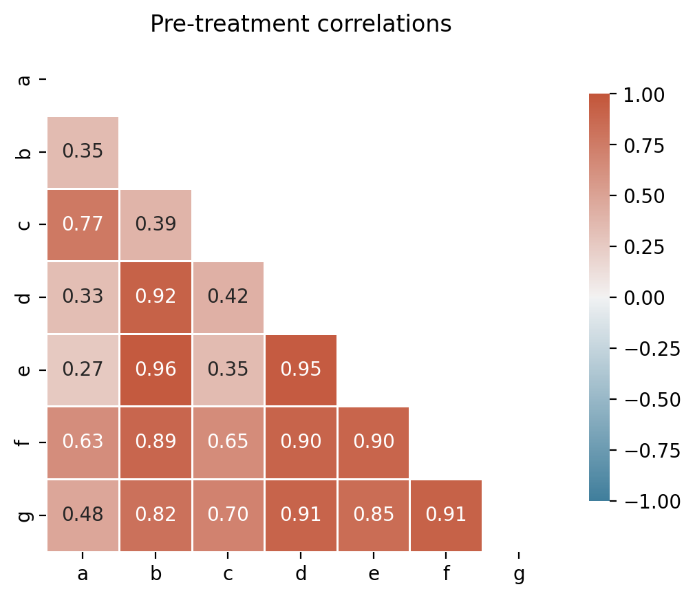
../_images/95bdda262d18e7faf22b1529e76a076e94ee664393c9f1f7c6f3defe6829eaab.png

All control units are positively correlated with the treated unit (actual), so no donor pool curation is needed for this dataset. In practice, you would exclude any controls with negative or near-zero correlations.

Run the analysis#

Note

The random_seed keyword argument for the PyMC sampler is not necessary. We use it here so that the results are reproducible.

Convex Hull Assumption#

The synthetic control method uses non-negative weights that sum to one. This means the synthetic control is a convex combination of the control units—it can only produce values within the range spanned by the controls at each time point.

Note

For the method to work well, the treated unit’s pre-intervention trajectory should lie within the “envelope” of the control units. If all controls are consistently above or below the treated unit, the method cannot construct an accurate counterfactual.

CausalPy automatically checks this assumption when you create a SyntheticControl object and will issue a warning if violated. See the Convex hull condition glossary entry and Abadie et al. [2010] for more details. The Augmented Synthetic Control Method [Ben-Michael et al., 2021] can handle cases where this assumption is violated.

df.head()

	a	b	c	d	e	f	g	counterfactual	causal effect	actual
0	0.793234	1.277264	-0.055407	-0.791535	1.075170	0.817384	-2.607528	0.144888	-0.0	0.398287
1	1.841898	1.185068	-0.221424	-1.430772	1.078303	0.890110	-3.108099	0.601862	-0.0	0.491644
2	2.867102	1.922957	-0.153303	-1.429027	1.432057	1.455499	-3.149104	1.060285	-0.0	1.232330
3	2.816255	2.424558	0.252894	-1.260527	1.938960	2.088586	-3.563201	1.520801	-0.0	1.672995
4	3.865208	2.358650	0.311572	-2.393438	1.977716	2.752152	-3.515991	1.983661	-0.0	1.775940

result = cp.SyntheticControl(
    df,
    treatment_time,
    control_units=["a", "b", "c", "d", "e", "f", "g"],
    treated_units=["actual"],
    model=cp.pymc_models.WeightedSumFitter(
        sample_kwargs={"target_accept": 0.95, "random_seed": seed}
    ),
)

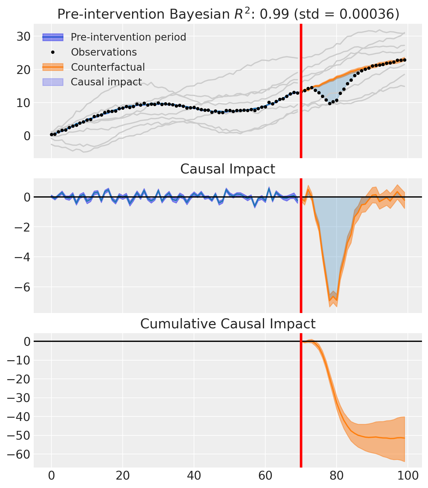
fig, ax = result.plot(plot_predictors=True)

../_images/0d006242a6993907ea42544f3828af8fd4a01627219e20961af599b221f4340d.png

result.summary()

================================SyntheticControl================================
Control units: ['a', 'b', 'c', 'd', 'e', 'f', 'g']
Treated unit: actual
Model coefficients:
    a            0.34, 94% HDI [0.3, 0.38]
    b            0.049, 94% HDI [0.01, 0.089]
    c            0.3, 94% HDI [0.26, 0.35]
    d            0.054, 94% HDI [0.0092, 0.099]
    e            0.026, 94% HDI [0.0015, 0.068]
    f            0.19, 94% HDI [0.1, 0.26]
    g            0.039, 94% HDI [0.0028, 0.09]
    y_hat_sigma  0.26, 94% HDI [0.22, 0.31]
Pre-treatment correlation (actual): 0.9961

As well as the model coefficients, we might be interested in the average causal impact and average cumulative causal impact.

az.summary(result.post_impact.mean("obs_ind"))

	mean	sd	hdi_3%	hdi_97%	mcse_mean	mcse_sd	ess_bulk	ess_tail	r_hat
x[actual]	-1.717	0.216	-2.133	-1.338	0.006	0.003	1260.0	1812.0	1.0

Warning

Care must be taken with the mean impact statistic. It only makes sense to use this statistic if it looks like the intervention had a lasting (and roughly constant) effect on the outcome variable. If the effect is transient, then clearly there will be a lot of post-intervention period where the impact of the intervention has ‘worn off’. If so, then it will be hard to interpret the mean impacts real meaning.

We can also ask for the summary statistics of the cumulative causal impact.

# get index of the final time point
index = result.post_impact_cumulative.obs_ind.max()
# grab the posterior distribution of the cumulative impact at this final time point
last_cumulative_estimate = result.post_impact_cumulative.sel({"obs_ind": index})
# get summary stats
az.summary(last_cumulative_estimate)

	mean	sd	hdi_3%	hdi_97%	mcse_mean	mcse_sd	ess_bulk	ess_tail	r_hat
x[actual]	-51.498	6.479	-63.982	-40.131	0.182	0.104	1260.0	1812.0	1.0

Effect Summary Reporting#

For decision-making, you often need a concise summary of the causal effect with key statistics. The effect_summary() method provides a decision-ready report with average and cumulative effects, HDI intervals, tail probabilities, and relative effects.

# Generate effect summary for the full post-period
stats = result.effect_summary(treated_unit="actual")
stats.table

	mean	median	hdi_lower	hdi_upper	p_gt_0	relative_mean	relative_hdi_lower	relative_hdi_upper
average	-1.716602	-1.706684	-2.147102	-1.326032	0.0	-9.124018	-11.221693	-7.261266
cumulative	-51.498075	-51.200525	-64.413068	-39.780954	0.0	-9.124018	-11.221693	-7.261266

print(stats.text)

During the post-period (70 to 99), the response variable had an average value of approx. 17.07. By contrast, in the absence of an intervention, we would have expected an average response of 18.79. The 95% interval of this counterfactual prediction is [18.40, 19.22]. Subtracting this prediction from the observed response yields an estimate of the causal effect the intervention had on the response variable. This effect is -1.72 with a 95% interval of [-2.15, -1.33].

Summing up the individual data points during the post-period, the response variable had an overall value of 512.18. By contrast, had the intervention not taken place, we would have expected a sum of 563.68. The 95% interval of this prediction is [551.97, 576.60].

The 95% HDI of the effect [-2.15, -1.33] does not include zero. The posterior probability of a decrease is 1.000. Relative to the counterfactual, the effect represents a -9.12% change (95% HDI [-11.22%, -7.26%]).

This analysis assumes that the control units used to construct the synthetic counterfactual were not themselves affected by the intervention, and that the pre-treatment relationship between control and treated units remains stable throughout the post-treatment period. We recommend inspecting model fit, examining pre-intervention trends, and conducting sensitivity analyses (e.g., placebo tests) to support any causal conclusions drawn from this analysis.

You can customize the summary in several ways:

Window: Analyze a specific time period instead of the full post-period
Direction: Specify whether you’re testing for an increase, decrease, or two-sided effect
Options: Include/exclude cumulative or relative effects

# Example: Analyze first half of post-period
post_indices = result.datapost.index
window_start = post_indices[0]
window_end = post_indices[len(post_indices) // 2]

stats_windowed = result.effect_summary(
    window=(window_start, window_end),
    treated_unit="actual",
    direction="two-sided",
    cumulative=True,
    relative=True,
)

stats_windowed.table

	mean	median	hdi_lower	hdi_upper	p_two_sided	prob_of_effect	relative_mean	relative_hdi_lower	relative_hdi_upper
average	-3.058950	-3.049049	-3.428534	-2.696519	0.0	1.0	-18.641865	-20.446211	-16.814846
cumulative	-48.943206	-48.784789	-54.856540	-43.144308	0.0	1.0	-18.641865	-20.446211	-16.814846

print(stats_windowed.text)

During the post-period (70 to 85), the response variable had an average value of approx. 13.34. By contrast, in the absence of an intervention, we would have expected an average response of 16.40. The 95% interval of this counterfactual prediction is [16.04, 16.77]. Subtracting this prediction from the observed response yields an estimate of the causal effect the intervention had on the response variable. This effect is -3.06 with a 95% interval of [-3.43, -2.70].

Summing up the individual data points during the post-period, the response variable had an overall value of 213.44. By contrast, had the intervention not taken place, we would have expected a sum of 262.38. The 95% interval of this prediction is [256.58, 268.30].

The 95% HDI of the effect [-3.43, -2.70] does not include zero. The posterior probability of a effect is 1.000. Relative to the counterfactual, the effect represents a -18.64% change (95% HDI [-20.45%, -16.81%]).

This analysis assumes that the control units used to construct the synthetic counterfactual were not themselves affected by the intervention, and that the pre-treatment relationship between control and treated units remains stable throughout the post-treatment period. We recommend inspecting model fit, examining pre-intervention trends, and conducting sensitivity analyses (e.g., placebo tests) to support any causal conclusions drawn from this analysis.

References#

[1] (1,2)

Alberto Abadie, Alexis Diamond, and Jens Hainmueller. Synthetic control methods for comparative case studies: estimating the effect of california's tobacco control program. Journal of the American Statistical Association, 105(490):493–505, 2010.

[2]

Alberto Abadie. Using synthetic controls: feasibility, data requirements, and methodological aspects. Journal of Economic Literature, 59(2):391–425, 2021.

[3]

Eli Ben-Michael, Ari Feller, and Jesse Rothstein. The augmented synthetic control method. Journal of the American Statistical Association, 116(536):1789–1803, 2021.

Synthetic control with pymc models#